Cohen's kappa: Learn it, use it, judge it

Imagine you have two friends trying to rate movies as either "good" or "bad." Now, think about a situation where they need to agree on the rating for 100 movies. That's where Cohen's kappa comes in - it measures how well they agree.

Similarly, let's say you have a machine learning model trying to predict if a person's credit is "good" or "bad" based on their financial history. You've got only human ratings for training the model. But the goal is for the model to operate independently in the future without the need for human ratings. Once the model is trained, we use Cohen's kappa to see how well the model and humans agree on these ratings. This helps you figure out the reliability of the model's predictions compared to human judgments and lets you determine the model's effectiveness in predicting creditworthiness.

It's like a tool that keeps track of how often everyone is on the same page. But here's the twist: it's not just about counting agreements, it considers the chance of random agreement too. So, when things get a bit tricky, and there's an unequal number of "good" and "bad" ratings, Cohen's kappa helps make sense of it all. It's like having a referee in the game of ratings, making sure everyone's on a fair playing field.

In this article we will:

• Guide you through the calculation and interpretation of Cohen’s kappa values, particularly in comparison with overall accuracy values
• Show that where overall accuracy fails because of a large imbalance in the class distribution, Cohen’s kappa might supply a more objective description of the model performance
• Introduce a few tips to keep in mind when interpreting Cohen’s kappa values!

Let’s look at classifying  bank loans, using the German credit data provided by the UCI Machine Learning Repository. The dataset has customers with either a “bad” credit rating (30%) or a “good” credit rating (70%) based on the bank’s criteria.  To highlight the imbalance, we adjusted the ratings to 10% "bad" and 90% "good" using bootstrapping. This creates a highly imbalanced dataset, helping us explain the difference between "overall accuracy" and "Cohen’s kappa" in this article.

Next, we’ll split the data into a training set (70%) and a test set (30%) using stratified sampling on the credit rating.We’ll then train a simple model like a decision tree. Due to the high levels of imbalance, the model may not perform well, but we’ll use the performance as the baseline for our study.

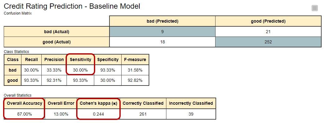
In figure 1 you can see the confusion matrix (a table to evaluate the performance of a classification model) and accuracy statistics for this baseline model. The overall accuracy of the model is quite high (87%) and hints at an acceptable performance by the model.

But when we look closer, we see that out of 30 people with bad credit, the model only got 9 of them right. That's not so good. The sensitivity value for the "bad" category is only 30%, which means it's not catching a lot of the people with bad credit

Basically, the decision tree is doing well in classifying the “good” customers correctly, but neglecting the few “bad” customers.  Even though the overall accuracy seems high, it's because there are a lot more "good" customers than "bad" ones.

To help us understand how well the model is doing beyond just accuracy, we look at Cohen's kappa value, which is 0.244 in this case. It's in a range from -1 to +1. The closer to +1, the better. So, 0.244 isn't great, indicating there's room for improvement in the model's performance.

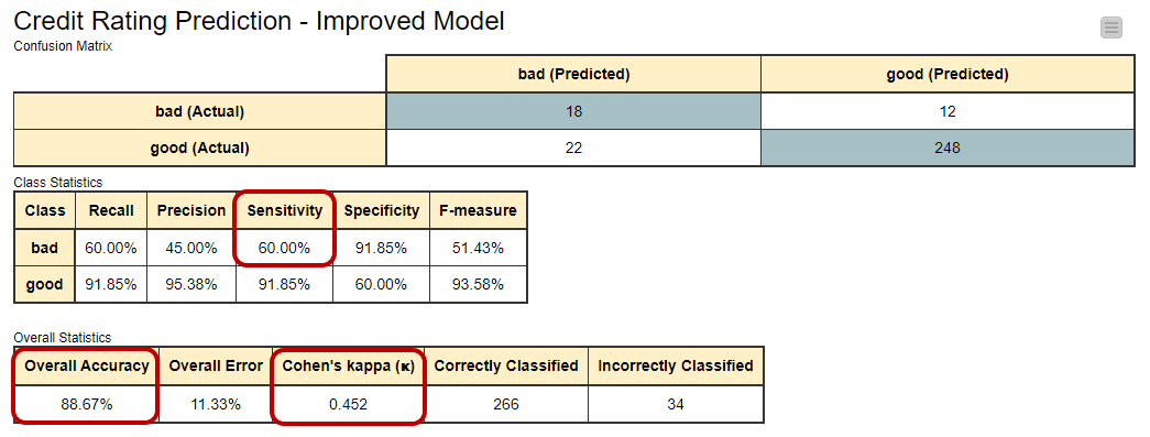
Let’s try to improve the model performance by forcing it to acknowledge the existence of the minority class i.e. the “bad” customers. We train the same model this time on a training set where the minority class has been oversampled using the SMOTE technique. This makes the dataset more balanced, with a 50-50 split between “good” and “bad” credit customers.  The improved model performs better on the minority class, correctly identifying 18 out of 30 customers with a "bad" credit rating. Cohen's kappa for this improved model increases to 0.452, showing a significant improvement in agreement. But what about overall accuracy? For this second model it’s 89%, not very different from the previous value 87%.

When summarizing we get two very different pictures. According to the overall accuracy, model performance hasn’t changed very much at all. However, according to Cohen’s kappa a lot has changed! Which statement is right?

From the numbers in the confusion matrix, it seems that Cohen’s kappa has a more realistic view of the model’s performance when using imbalanced data.

• Why does Cohen’s kappa take more notice of the minority class? How is it actually calculated? Let’s take a look!

Cohen’s kappa is calculated with the following formula [1]:

where p0 is the overall accuracy of the model and pe represents the agreement between the model predictions and the actual class values as if happening by chance.

In a binary classification problem, like ours, pe is the sum of pe1, the probability of the predictions agreeing with actual values of class 1 (“good”) by chance, and pe2, the probability of the predictions agreeing with the actual values of class 2 (“bad”) by chance. Assuming that the two classifiers - model predictions and actual class values - are independent, these probabilities, pe1 and pe2, are calculated by multiplying the proportion of the actual class and the proportion of the predicted class.

If we consider “bad” as the positive class, the baseline model (Figure 1) assigned 9% of the records (false positives plus true positives) to class “bad”, and 91% of the records (true negatives plus false negatives) to class “good”. Thus pe is:

And therefore Cohen’s kappa statistics:

which is the same value as reported in figure 1.

In simple terms, Cohen's kappa helps us evaluate a classifier by considering how often it makes predictions that go beyond random chance. 

At this point, we know that Cohen’s kappa is a useful evaluation metric when dealing with imbalanced data. However, Cohen’s kappa has some downsides, too. Let’s have a look at them one by one.

It’s easier to reach higher values of Cohen’s kappa, if the target class distribution is balanced.

For the baseline model (Figure 1), the distribution of the predicted classes follows closely the distribution of the target classes: 27 predicted as “bad” vs. 273 predicted as “good” and 30 being actually “bad” vs. 270 being actually “good”.

For the improved model (Figure 2), the difference between the two class distributions is greater: 40 predicted as “bad” vs. 260 predicted as “good” and 30 being actually “bad” vs. 270 being actually “good”.

As the formula for maximum Cohen’s kappa shows, the more the distributions of the predicted and actual target classes differ, the lower the maximum reachable Cohen’s kappa value is. The maximum Cohen’s kappa value represents the edge case of either the number of false negatives or false positives in the confusion matrix being zero, i.e. all customers with a good credit rating, or alternatively all customers with a bad credit rating, are predicted correctly.

where pmax is the maximum reachable overall accuracy of the model given the distributions of the target and predicted classes:

For the baseline model, we get the following value for pmax:

Whereas for the improved model it is:

The maximum value of Cohen’s kappa is then for the baseline model:

For the improved model it is:

As the results show, the improved model with a greater difference in the distributions between the actual and predicted target classes can only reach a Cohen's kappa value as high as 0.853. Whereas the baseline model can reach the value 0.942, despite the worse performance.

When we calculate Cohen’s kappa, we strongly assume that the distributions of target and predicted classes are independent and that the target class doesn’t affect the probability of a correct prediction. In our example this would mean that a credit customer with a good credit rating has an equal chance of getting a correct prediction as a credit customer with a bad credit rating. However, since we know that our baseline model is biased towards the majority “good” class , this assumption is violated.

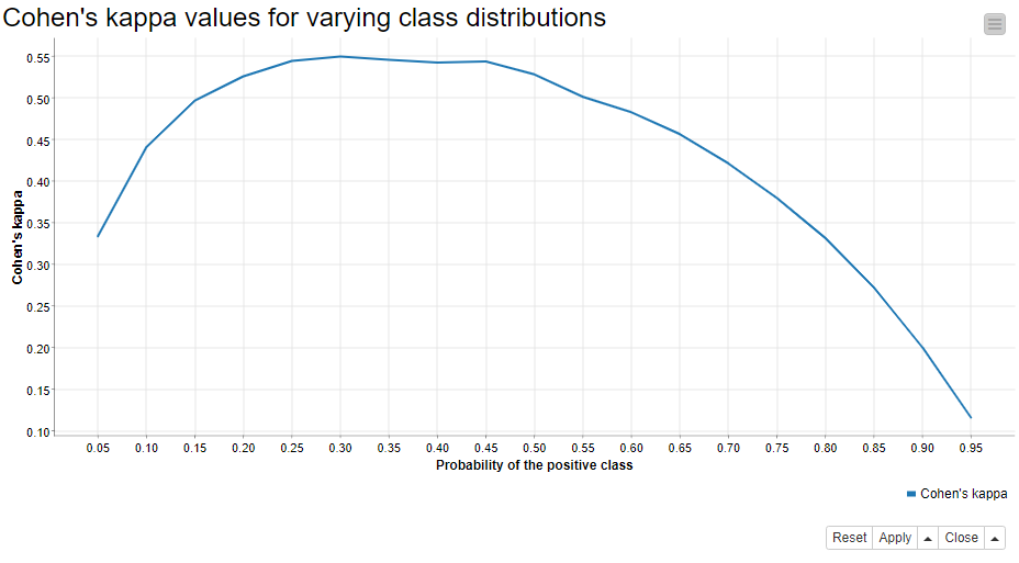
If this assumption were not violated, like in the improved model where the target classes are balanced, we could reach higher values of Cohen’s kappa. Why is this? We can rewrite the formula of Cohen’s kappa as the function of the probability of the positive class, and the function reaches its maximum when the probability of the positive class is 0.5 [1]. We test this by applying the same improved model (figure 2) to different test sets, where the proportion of the positive “bad” class varies between 5% and 95%. We create 100 different test sets per class distribution by bootstrapping the original test data, and calculate the average Cohen’s kappa value from the results.

Figure 3 shows the average Cohen’s kappa values against the positive class probabilities - and yes! Cohen’s kappa does reach its maximum when the model is applied to balanced data!

The numerator of Cohen’s kappa, p0-pe, tells the difference between the observed overall accuracy of the model and the overall accuracy that can be obtained by chance. The denominator of the formula, 1-pe, tells the maximum value for this difference.

For a good model, the observed difference and the maximum difference are close to each other, and Cohen’s kappa is close to 1. For a random model, the overall accuracy is all due to the random chance, the numerator is 0, and Cohen’s kappa is 0. Cohen’s kappa could also theoretically be negative. Then, the overall accuracy of the model would be even lower than what could have been obtained by a random guess.

Given the explanation above, Cohen’s kappa is not easy to interpret in terms of an expected accuracy, and it’s often not recommended to follow any verbal categories as interpretations. For example, if you have 100 customers and a model with an overall accuracy of 87 %, then you can expect to predict the credit rating correctly for 87 customers. Cohen’s kappa value 0.244 doesn’t provide you with an interpretation as easy as this.

In this article we have explained how to use and interpret Cohen’s kappa to evaluate the performance of a classification model. While Cohen’s kappa can correct the bias of overall accuracy when dealing with unbalanced data, it has a few shortcomings. So the next time you take a look at the scoring metrics of your model, remember:

1. Cohen’s kappa is more informative than overall accuracy when working with imbalanced data. Keep this in mind when you compare or optimize classification models!
2. Take a look at the row and column totals in the confusion matrix. Are the distributions of the target/predicted classes similar? If they’re not, the maximum reachable Cohen’s kappa value will be lower.
3. The same model will give you lower values of Cohen’s kappa for imbalanced than for balanced test data.
4. Cohen’s kappa says little about the expected accuracy of a single prediction.

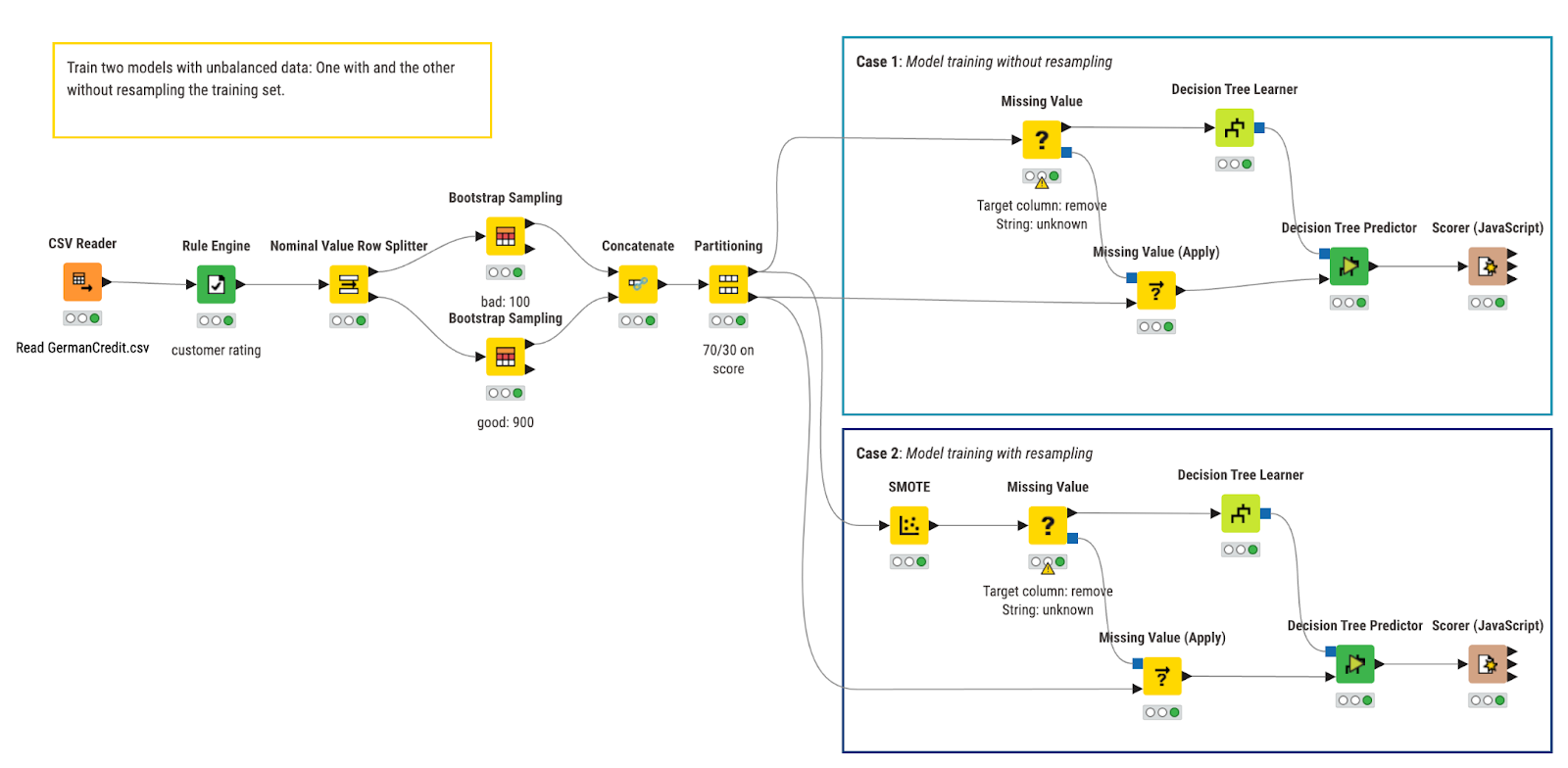
The workflow used for this study is shown in Figure 4. In the workflow we train, apply, and evaluate two decision tree models that predict the creditworthiness of credit customers. In the top branch, we train the baseline model, while in the bottom branch we train the model on the bootstrapped training set using the SMOTE technique.

• Download the workflow from the Cohen’s Kappa for Evaluating Classification Models page on the KNIME Hub.

[1] Bland, Martin. "Cohen’s kappa." University of York Department of Health Sciences https://www-users.york.ac.uk/~mb55/msc/clinimet/week4/kappa_text.pdf. [Accessed May 29 2020] (2008).

As first published in The New Stack.